Plot confidence intervals for a fastcpd object

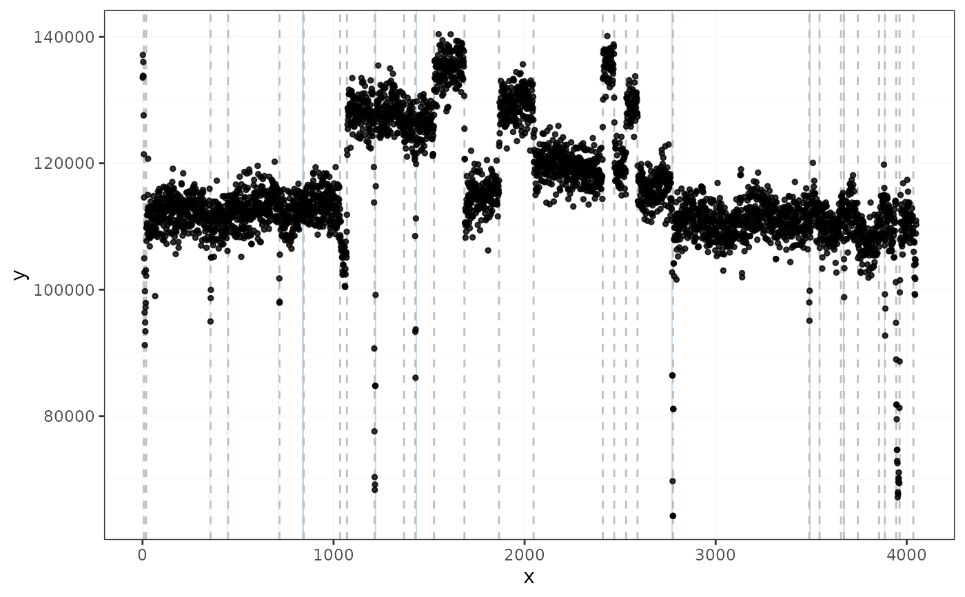
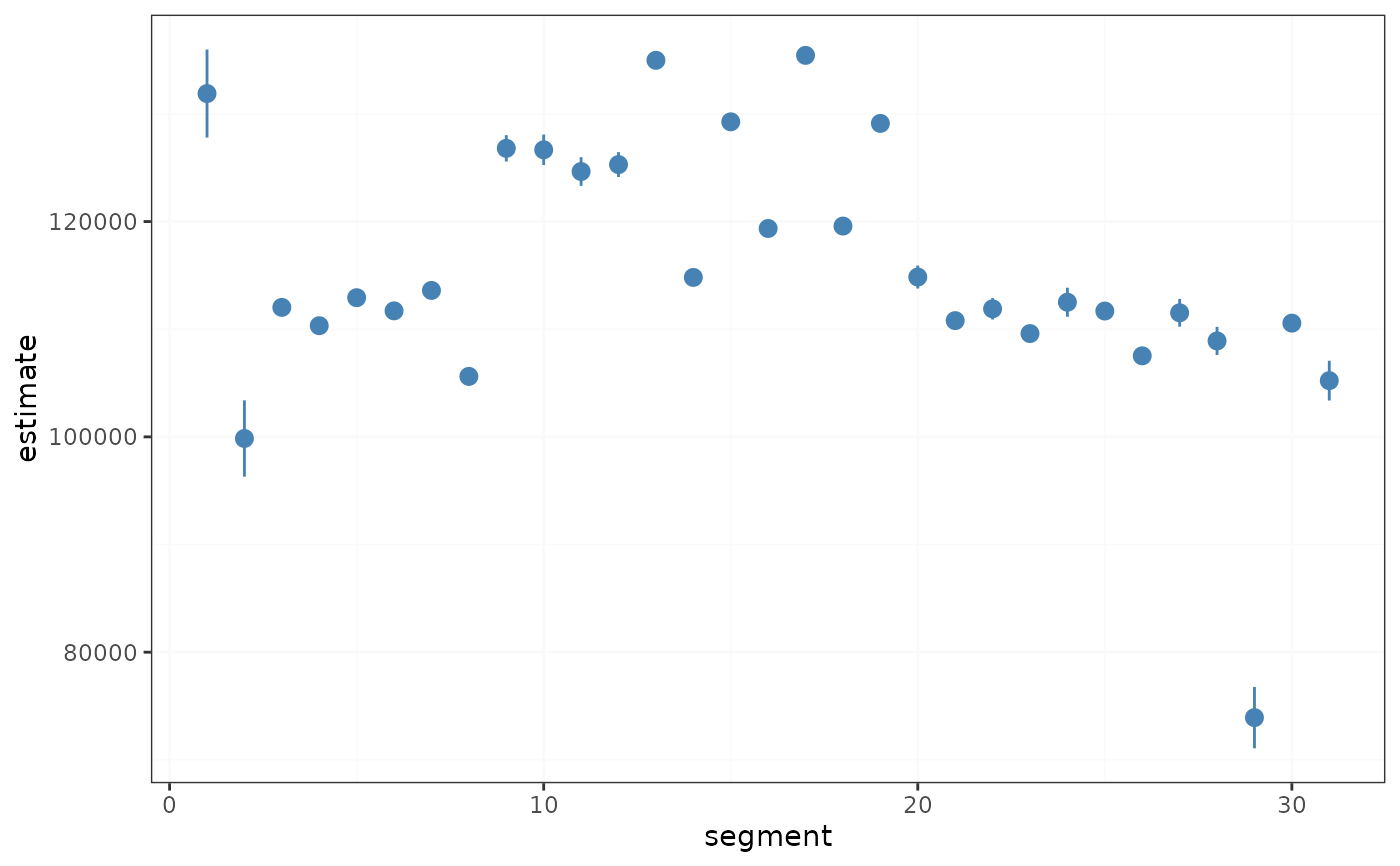
Visualizes intervals produced by confint.fastcpd(). Change-point intervals are drawn as shaded bands over the data with the point estimates as vertical lines. Parameter intervals are drawn as point ranges for each segment, with one panel per parameter.

Plotting change-point intervals requires the fitted object stored on the fastcpd_confint data frame, so pass the value returned by confint() without subsetting it.

Usage

# S3 method for class 'fastcpd_confint'
plot(
  x,
  data_point_alpha = 0.8,
  data_point_linewidth = 0.5,
  data_point_size = 1,
  interval_alpha = 0.3,
  interval_color = "steelblue",
  estimate_color = "grey",
  estimate_linetype = "dashed",
  xlab = NULL,
  ylab = NULL,
  ...
)

Arguments

x

A fastcpd_confint data frame returned by confint.fastcpd().

data_point_alpha

Alpha of the data points.

data_point_linewidth

Linewidth of the data lines.

data_point_size

Size of the data points.

interval_alpha

Alpha of the confidence interval bands.

interval_color

Color of the confidence intervals.

estimate_color

Color of the point-estimate lines.

estimate_linetype

Linetype of the point-estimate lines.

xlab

Label for the x-axis.

ylab

Label for the y-axis.

...

Ignored.

Value

No return value, called for plotting.

Examples

sigma2 <- estimate_variance_median(well_log)
result <- detect_mean(well_log, trim = 0.001, variance_estimation = sigma2)

cp_profile_interval <- confint(
  result,
  parm = "cp",
  method = "profile",
  level = 0.8,
  window = 8
)
plot(cp_profile_interval)


theta_wald_interval <- confint(result, parm = "theta", method = "wald")
plot(theta_wald_interval)